Getting familiar with dplyr

Feb 11, 2020 26 min read R

The aim of this workshop is to get familiar with dplyr, an R package to transform and summarize dataframe.

The packages lubridate will be sligtly described

your_dataset<- read.csv("~/Dropbox/folder1/folder2/awesomedata.csv") # how to read your file
bike<-readRDS("~/folder1/folder2/trips.RDS") # here is the dataset I'm using as an example. 
# don't forget to copy your own path !!
library(dplyr)
library(lubridate)

Description of the database “bike”

trips is a dataset containing information on each bike rental:

Variable Name	Description
Duration	duration of the trip in seconds
Start.date	time stamp of the return date and time. Date is collected as year, month, and day; time is written as hour, minute, and seconds.
End.date	time stamp of the return date and time. Same format as `Start.date`.
Start.station.number	station identifier of the station the bike was checked out.
Start.station	station name of the station the bike was checked out.
End.station.number	station identifier of the station the bike was returned to.
End.station	station name of the station the bike was returned to.
Bike.number	bike identifier.
Member.type	Member or Casual - type of membership of the renter.

dim(bike) # dimension of your dataset
## [1] 815370      9
str(bike) # structure of your dataset
## 'data.frame':    815370 obs. of  9 variables:
##  $ Duration            : num  197 435 955 462 3357 ...
##  $ Start.date          : Factor w/ 735188 levels "2017-10-01 00:00:02",..: 1 2 3 3 4 5 6 7 8 9 ...
##  $ End.date            : Factor w/ 734389 levels "2017-10-01 00:03:19",..: 1 2 19 3 120 71 21 6 9 9 ...
##  $ Start.station.number: Factor w/ 488 levels "31000","31001",..: 144 105 151 112 190 190 291 215 103 210 ...
##  $ Start.station       : Factor w/ 488 levels "10th & E St NW",..: 59 167 67 6 106 106 84 103 12 15 ...
##  $ End.station.number  : Factor w/ 488 levels "31000","31001",..: 159 290 104 103 190 219 189 132 267 270 ...
##  $ End.station         : Factor w/ 488 levels "10th & E St NW",..: 361 377 55 12 106 282 95 50 258 87 ...
##  $ Bike.number         : Factor w/ 4293 levels "W00005","W00007",..: 2157 381 1450 2149 3297 2227 592 3400 736 401 ...
##  $ Member.type         : Factor w/ 2 levels "Casual","Member": 2 2 2 2 1 1 1 2 2 2 ...
head(bike) # returns the first part of your dataset
##   Duration          Start.date            End.date Start.station.number
## 1  197.068 2017-10-01 00:00:02 2017-10-01 00:03:19                31214
## 2  434.934 2017-10-01 00:00:23 2017-10-01 00:07:38                31104
## 3  955.437 2017-10-01 00:00:56 2017-10-01 00:16:52                31221
## 4  461.619 2017-10-01 00:00:56 2017-10-01 00:08:37                31111
## 5 3357.184 2017-10-01 00:00:59 2017-10-01 00:56:56                31260
## 6 2235.414 2017-10-01 00:01:06 2017-10-01 00:38:21                31260
##                 Start.station End.station.number
## 1       17th & Corcoran St NW              31229
## 2 Adams Mill & Columbia Rd NW              31602
## 3              18th & M St NW              31103
## 4              10th & U St NW              31102
## 5             23rd & E St NW               31260
## 6             23rd & E St NW               31289
##                                   End.station Bike.number Member.type
## 1                 New Hampshire Ave & T St NW      W21022      Member
## 2                     Park Rd & Holmead Pl NW      W00470      Member
## 3                        16th & Harvard St NW      W20206      Member
## 4                         11th & Kenyon St NW      W21014      Member
## 5                             23rd & E St NW       W22349      Casual
## 6 Henry Bacon Dr & Lincoln Memorial Circle NW      W21107      Casual

chaining functions

The pipe operator in R, represented by %>% can be used to chain code together.

You take the output of one function and send it directly to the next

%>% can be read as “then”

Important dplyr verbs

FILTER

filter rows

example: filter by casual member type

bike %>% filter(Member.type=="Casual") %>% head()
##   Duration          Start.date            End.date Start.station.number
## 1 3357.184 2017-10-01 00:00:59 2017-10-01 00:56:56                31260
## 2 2235.414 2017-10-01 00:01:06 2017-10-01 00:38:21                31260
## 3 1177.391 2017-10-01 00:01:14 2017-10-01 00:20:51                31603
## 4 1268.953 2017-10-01 00:06:12 2017-10-01 00:27:21                31240
## 5 1241.639 2017-10-01 00:06:18 2017-10-01 00:27:00                31240
## 6 1248.658 2017-10-01 00:06:26 2017-10-01 00:27:15                31240
##                                      Start.station End.station.number
## 1                                  23rd & E St NW               31260
## 2                                  23rd & E St NW               31289
## 3                                    1st & M St NE              31259
## 4 Ohio Dr & West Basin Dr SW / MLK & FDR Memorials              31258
## 5 Ohio Dr & West Basin Dr SW / MLK & FDR Memorials              31258
## 6 Ohio Dr & West Basin Dr SW / MLK & FDR Memorials              31258
##                                   End.station Bike.number Member.type
## 1                             23rd & E St NW       W22349      Casual
## 2 Henry Bacon Dr & Lincoln Memorial Circle NW      W21107      Casual
## 3                   20th St & Virginia Ave NW      W00708      Casual
## 4                            Lincoln Memorial      W01106      Casual
## 5                            Lincoln Memorial      W21442      Casual
## 6                            Lincoln Memorial      W21731      Casual

You can filter using the boolean operators (e.g. >, <, >=, <=, !=, %in%) to create the logical tests.

bike %>% filter(Duration>=1000) 

bike %>% filter(Member.type=="Casual", 
                Duration>=1000) 

bike %>% filter(Member.type=="Casual", 
                Start.station %in% c("Lincoln Memorial","6th & K St NE","Kennedy Center"))

%in% operator in R, is used to identify if an element belongs to a vector.

filter without dplyr :(

bike[bike$Member.type=="Casual" & bike$Duration>=1000,]

SELECT

select columns

example: how to select two columns?

bike %>% select(Start.station,End.station) %>% head()

select a group of columns: use “:” operator

bike %>% select(Duration:End.station)

select all the columns except specific columns: use the “-” operator

bike %>% select(-Bike.number,-Member.type)

select all the columns except a group of columns: : use the “-” and “:” operators

bike %>% select(-(Duration:End.station))

select columns based on a character experession

bike %>% select(contains('station')) %>% head()
##   Start.station.number               Start.station End.station.number
## 1                31214       17th & Corcoran St NW              31229
## 2                31104 Adams Mill & Columbia Rd NW              31602
## 3                31221              18th & M St NW              31103
## 4                31111              10th & U St NW              31102
## 5                31260             23rd & E St NW               31260
## 6                31260             23rd & E St NW               31289
##                                   End.station
## 1                 New Hampshire Ave & T St NW
## 2                     Park Rd & Holmead Pl NW
## 3                        16th & Harvard St NW
## 4                         11th & Kenyon St NW
## 5                             23rd & E St NW 
## 6 Henry Bacon Dr & Lincoln Memorial Circle NW

select without dplyr :(

bike[,c("Start.station","End.station")]

RENAME

rename column’s name

bike %>% rename(Bike_ID=Bike.number) %>% head()
##   Duration          Start.date            End.date Start.station.number
## 1  197.068 2017-10-01 00:00:02 2017-10-01 00:03:19                31214
## 2  434.934 2017-10-01 00:00:23 2017-10-01 00:07:38                31104
## 3  955.437 2017-10-01 00:00:56 2017-10-01 00:16:52                31221
## 4  461.619 2017-10-01 00:00:56 2017-10-01 00:08:37                31111
## 5 3357.184 2017-10-01 00:00:59 2017-10-01 00:56:56                31260
## 6 2235.414 2017-10-01 00:01:06 2017-10-01 00:38:21                31260
##                 Start.station End.station.number
## 1       17th & Corcoran St NW              31229
## 2 Adams Mill & Columbia Rd NW              31602
## 3              18th & M St NW              31103
## 4              10th & U St NW              31102
## 5             23rd & E St NW               31260
## 6             23rd & E St NW               31289
##                                   End.station Bike_ID Member.type
## 1                 New Hampshire Ave & T St NW  W21022      Member
## 2                     Park Rd & Holmead Pl NW  W00470      Member
## 3                        16th & Harvard St NW  W20206      Member
## 4                         11th & Kenyon St NW  W21014      Member
## 5                             23rd & E St NW   W22349      Casual
## 6 Henry Bacon Dr & Lincoln Memorial Circle NW  W21107      Casual

hint

database_name %>% rename(new_column_name = old_column_name)

ARRANGE

arrange or re-order row by a specific column

example: arrange by duration ** ascending order

bike %>%
  select(Start.station,Duration) %>%
  arrange(Duration) %>% 
  head()
##                 Start.station Duration
## 1               1st & M St NE   60.025
## 2               8th & O St NW   60.041
## 3    18th St & Wyoming Ave NW   60.062
## 4              14th & D St SE   60.069
## 5 Mount Vernon Ave & Bruce St   60.083
## 6              15th & P St NW   60.089

use severals columns to arrange rows

bike %>%
  select(Start.station,Duration) %>%
  arrange(Start.station,Duration) %>% 
  head()
##    Start.station Duration
## 1 10th & E St NW   75.117
## 2 10th & E St NW   77.270
## 3 10th & E St NW   80.548
## 4 10th & E St NW   81.516
## 5 10th & E St NW   81.975
## 6 10th & E St NW   82.647

Here, you arrange first by start station and then by duration

descending order: use “desc”

bike %>%
  select(Start.station,Duration) %>%
  arrange(desc(Duration)) %>%
  head()
##                                 Start.station Duration
## 1              15th St & Massachusetts Ave SE 86275.45
## 2              15th St & Massachusetts Ave SE 86267.48
## 3              L'Enfant Plaza / 7th & C St SW 85881.14
## 4 Henry Bacon Dr & Lincoln Memorial Circle NW 85021.03
## 5                 Columbia Rd & Belmont St NW 84938.20
## 6            Constitution Ave & 2nd St NW/DOL 84915.39

arrange sans dplyr :(

bike[order(bike$Duration),c("Start.station","Duration")]

JOIN

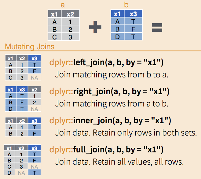
use join() for joining datasets. In dplyr there are several join functions left_join right_join full_join inner_join

df1 <- data.frame(id = 1:6, trt = rep(c("A", "B", "C"), rep=c(2,1,3)), value = c(5,3,7,1,2,3))
df1
##   id trt value
## 1  1   A     5
## 2  2   B     3
## 3  3   C     7
## 4  4   A     1
## 5  5   B     2
## 6  6   C     3

df2 <- data.frame(id=c(4,4,5,5,7,7), stress=rep(c(0,1), 3), bpm = c(65, 125, 74, 136, 48, 110))
df2
##   id stress bpm
## 1  4      0  65
## 2  4      1 125
## 3  5      0  74
## 4  5      1 136
## 5  7      0  48
## 6  7      1 110

left_join & right_join

all elements in the left data set are kept
non-matched are filled in by NA
right_join works symmetric

left_join(df1,df2,by="id")
##   id trt value stress bpm
## 1  1   A     5     NA  NA
## 2  2   B     3     NA  NA
## 3  3   C     7     NA  NA
## 4  4   A     1      0  65
## 5  4   A     1      1 125
## 6  5   B     2      0  74
## 7  5   B     2      1 136
## 8  6   C     3     NA  NA

right_join(df1,df2,by="id")
##   id  trt value stress bpm
## 1  4    A     1      0  65
## 2  4    A     1      1 125
## 3  5    B     2      0  74
## 4  5    B     2      1 136
## 5  7 <NA>    NA      0  48
## 6  7 <NA>    NA      1 110

inner_join

only matches from both data sets are kept

inner_join(df1, df2, by = "id")
##   id trt value stress bpm
## 1  4   A     1      0  65
## 2  4   A     1      1 125
## 3  5   B     2      0  74
## 4  5   B     2      1 136

full_join

all ids are kept, missings are filled in with NA

full_join(df1, df2, by = "id")
##    id  trt value stress bpm
## 1   1    A     5     NA  NA
## 2   2    B     3     NA  NA
## 3   3    C     7     NA  NA
## 4   4    A     1      0  65
## 5   4    A     1      1 125
## 6   5    B     2      0  74
## 7   5    B     2      1 136
## 8   6    C     3     NA  NA
## 9   7 <NA>    NA      0  48
## 10  7 <NA>    NA      1 110

anti_join

return all rows from df1 where there are not matching values in df2, keeping just columns from df1.
be careful is not symmetric!

anti_join(df1,df2,by="id")
##   id trt value
## 1  1   A     5
## 2  2   B     3
## 3  3   C     7
## 4  6   C     3

MUTATE

mutate allows us to introduce new variables or upgrade existing ones
The result from mutate are vectors of the same length as teh data set

create a column called “Duration_min” which is the duration in minutes

bike %>% mutate(Duration_min = Duration/60) %>% head()
##   Duration          Start.date            End.date Start.station.number
## 1  197.068 2017-10-01 00:00:02 2017-10-01 00:03:19                31214
## 2  434.934 2017-10-01 00:00:23 2017-10-01 00:07:38                31104
## 3  955.437 2017-10-01 00:00:56 2017-10-01 00:16:52                31221
## 4  461.619 2017-10-01 00:00:56 2017-10-01 00:08:37                31111
## 5 3357.184 2017-10-01 00:00:59 2017-10-01 00:56:56                31260
## 6 2235.414 2017-10-01 00:01:06 2017-10-01 00:38:21                31260
##                 Start.station End.station.number
## 1       17th & Corcoran St NW              31229
## 2 Adams Mill & Columbia Rd NW              31602
## 3              18th & M St NW              31103
## 4              10th & U St NW              31102
## 5             23rd & E St NW               31260
## 6             23rd & E St NW               31289
##                                   End.station Bike.number Member.type
## 1                 New Hampshire Ave & T St NW      W21022      Member
## 2                     Park Rd & Holmead Pl NW      W00470      Member
## 3                        16th & Harvard St NW      W20206      Member
## 4                         11th & Kenyon St NW      W21014      Member
## 5                             23rd & E St NW       W22349      Casual
## 6 Henry Bacon Dr & Lincoln Memorial Circle NW      W21107      Casual
##   Duration_min
## 1     3.284467
## 2     7.248900
## 3    15.923950
## 4     7.693650
## 5    55.953067
## 6    37.256900

LUBRIDATE

Your best friend to work with dates and times

You need to call library(lubridate) or library(tidyverse)

Most of the time dates are in character format. Lubridate will help you to parse your dates.
For example: * ymd() converts dates in year-month-day * dmy() converts dates in day-month-year * ydm() converts dates in year-day-month

examples

mdy("3/27/2018") 
## [1] "2018-03-27"
dmy("27/3/2018")
## [1] "2018-03-27"
class(mdy("3/27/2018"))
## [1] "Date"
class("3/27/2018")
## [1] "character"

also works when month is written in letters

mdy("JAN-10-2019")
## [1] "2019-01-10"
mdy("March-10-2006")
## [1] "2006-03-10"

different ways to print the dates

today<-mdy("12/05/2019")
month(today)                       # numeric
## [1] 12
month(today,label=TRUE)            # character 
## [1] Dec
## 12 Levels: Jan < Feb < Mar < Apr < May < Jun < Jul < Aug < Sep < ... < Dec
month(today,label=TRUE,abbr=FALSE) # character and without abbreviation
## [1] December
## 12 Levels: January < February < March < April < May < June < ... < December
wday(today,label=TRUE,abbr=FALSE)  # same but for the day
## [1] Thursday
## 7 Levels: Sunday < Monday < Tuesday < Wednesday < Thursday < ... < Saturday

You can work with upcoming dates

christmas<-mdy("12/25/2019")
wday(christmas,label=TRUE,abbr= F) 
## [1] Wednesday
## 7 Levels: Sunday < Monday < Tuesday < Wednesday < Thursday < ... < Saturday

parse times (hour, minutes, secondes)

ymd_hms("2018-03-27 15:09:28")
## [1] "2018-03-27 15:09:28 UTC"
hour(ymd_hms("2018-03-27 15:09:28"))
## [1] 15

Using mutate we can create new variables returning the day, month and week for example

bike<- bike %>%  
  mutate(
    Start.date = ydm_hms(Start.date), # first parse the date 
    weekday=wday(Start.date,label=TRUE),
    month=month(Start.date,label=TRUE),
    week= week(Start.date)
  )
head(bike)
##   Duration          Start.date            End.date Start.station.number
## 1  197.068 2017-01-10 00:00:02 2017-10-01 00:03:19                31214
## 2  434.934 2017-01-10 00:00:23 2017-10-01 00:07:38                31104
## 3  955.437 2017-01-10 00:00:56 2017-10-01 00:16:52                31221
## 4  461.619 2017-01-10 00:00:56 2017-10-01 00:08:37                31111
## 5 3357.184 2017-01-10 00:00:59 2017-10-01 00:56:56                31260
## 6 2235.414 2017-01-10 00:01:06 2017-10-01 00:38:21                31260
##                 Start.station End.station.number
## 1       17th & Corcoran St NW              31229
## 2 Adams Mill & Columbia Rd NW              31602
## 3              18th & M St NW              31103
## 4              10th & U St NW              31102
## 5             23rd & E St NW               31260
## 6             23rd & E St NW               31289
##                                   End.station Bike.number Member.type weekday
## 1                 New Hampshire Ave & T St NW      W21022      Member     Tue
## 2                     Park Rd & Holmead Pl NW      W00470      Member     Tue
## 3                        16th & Harvard St NW      W20206      Member     Tue
## 4                         11th & Kenyon St NW      W21014      Member     Tue
## 5                             23rd & E St NW       W22349      Casual     Tue
## 6 Henry Bacon Dr & Lincoln Memorial Circle NW      W21107      Casual     Tue
##   month week
## 1   Jan    2
## 2   Jan    2
## 3   Jan    2
## 4   Jan    2
## 5   Jan    2
## 6   Jan    2

tip: don’t forget to save the new variables using “bike <-”

SUMMARISE

summarise() function create summary statistics for a given column (such as the mean, sd).

compute the average duration of trips, apply the mean() function to the column duration

bike %>% 
  summarise(avg_duration=mean(Duration/60))  
##   avg_duration
## 1     16.56157

SUMMARISE & GROUP_BY

group_by splits the data into groups.
group_by introduces structure to a data set

What is the average duration of trips (minutes) per member type?

bike %>% 
  group_by(Member.type) %>%
  summarise(avg_duration=mean(Duration/60))   
## # A tibble: 2 x 2
##   Member.type avg_duration
##   <fct>              <dbl>
## 1 Casual              36.1
## 2 Member              11.9

summarise() returns a single-row summary for each group

What is the total number of trips per weekday?

bike %>% 
  group_by(weekday) %>%
  summarise(nbtrips=n())  #n() returns the number of observations within a group
## Warning: Factor `weekday` contains implicit NA, consider using
## `forcats::fct_explicit_na`
## # A tibble: 8 x 2
##   weekday nbtrips
##   <ord>     <int>
## 1 Mon       53068
## 2 Tue       49620
## 3 Wed       49122
## 4 Thu       30101
## 5 Fri       54111
## 6 Sat       55066
## 7 Sun       53926
## 8 <NA>     470356

hint: count() is a shortcut for group_by() + n()

example with count()

bike %>% count(weekday)  
## Warning: Factor `weekday` contains implicit NA, consider using
## `forcats::fct_explicit_na`
## # A tibble: 8 x 2
##   weekday      n
##   <ord>    <int>
## 1 Mon      53068
## 2 Tue      49620
## 3 Wed      49122
## 4 Thu      30101
## 5 Fri      54111
## 6 Sat      55066
## 7 Sun      53926
## 8 <NA>    470356

What is the total number of trips per weekday and per member type?

bike %>% 
  na.omit() %>% # remove NA
  group_by(weekday,Member.type) %>%
  summarise(nbtrips=n())
## # A tibble: 14 x 3
## # Groups:   weekday [7]
##    weekday Member.type nbtrips
##    <ord>   <fct>         <int>
##  1 Mon     Casual        12353
##  2 Mon     Member        40715
##  3 Tue     Casual        11657
##  4 Tue     Member        37963
##  5 Wed     Casual         5859
##  6 Wed     Member        43263
##  7 Thu     Casual         7764
##  8 Thu     Member        22337
##  9 Fri     Casual         6874
## 10 Fri     Member        47237
## 11 Sat     Casual        10913
## 12 Sat     Member        44153
## 13 Sun     Casual         9932
## 14 Sun     Member        43994

data visualization

bike %>% 
  na.omit() %>% # remove NA
  group_by(weekday,Member.type) %>%
  summarise(nbtrips=n()) %>%
  ggplot(aes(x=weekday,weight=nbtrips)) + 
  geom_bar() + 
  facet_grid(~Member.type)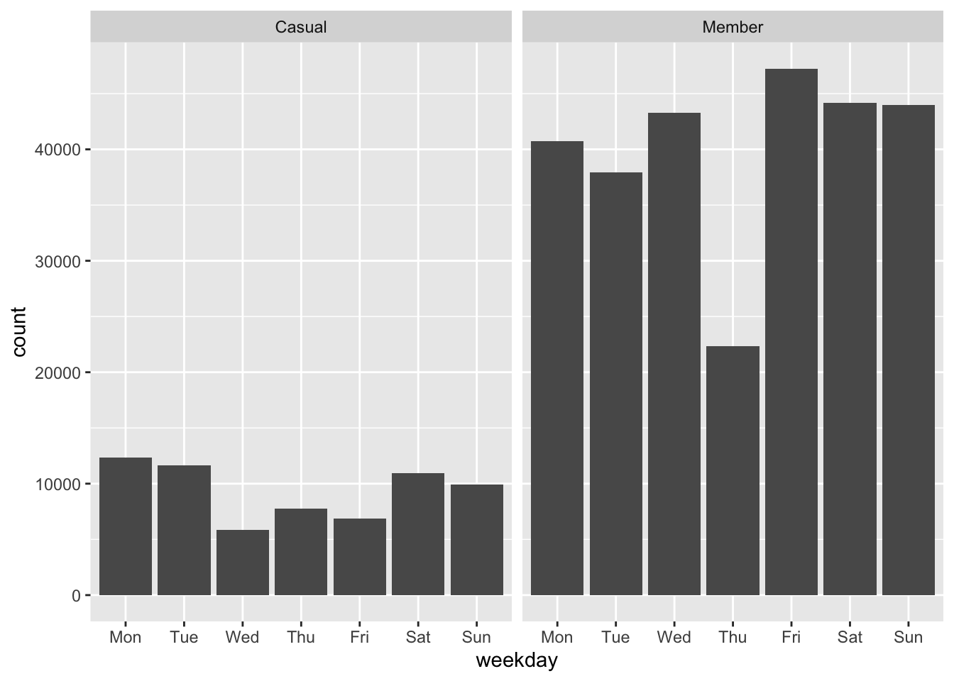

For the following start stations:

Lincoln Memorial,6th & K St NE,Kennedy Center.

What is the average duration of trips in minutes?

Return the result by ascending order

bike %>% 
  filter (Start.station %in% c("Lincoln Memorial","6th & K St NE","Kennedy Center")) %>%
  group_by(Start.station) %>%
  summarise(mean_duration=(mean(Duration/60, na.rm=TRUE))) %>% 
  arrange(mean_duration)
## # A tibble: 3 x 2
##   Start.station    mean_duration
##   <fct>                    <dbl>
## 1 6th & K St NE             14.1
## 2 Kennedy Center            20.6
## 3 Lincoln Memorial          33.7

SUMMARISE_ALL

use summarise_all to apply a function to multiple variables

Example with the database iris

head(iris)
##   Sepal.Length Sepal.Width Petal.Length Petal.Width Species
## 1          5.1         3.5          1.4         0.2  setosa
## 2          4.9         3.0          1.4         0.2  setosa
## 3          4.7         3.2          1.3         0.2  setosa
## 4          4.6         3.1          1.5         0.2  setosa
## 5          5.0         3.6          1.4         0.2  setosa
## 6          5.4         3.9          1.7         0.4  setosa

iris %>% 
  group_by(Species) %>%
  summarise_all(mean)
## # A tibble: 3 x 5
##   Species    Sepal.Length Sepal.Width Petal.Length Petal.Width
##   <fct>             <dbl>       <dbl>        <dbl>       <dbl>
## 1 setosa             5.01        3.43         1.46       0.246
## 2 versicolor         5.94        2.77         4.26       1.33 
## 3 virginica          6.59        2.97         5.55       2.03

to apply multiple transformations, use funs()

iris %>%
  group_by(Species) %>%
  summarise_all(funs(min,max))
## # A tibble: 3 x 9
##   Species Sepal.Length_min Sepal.Width_min Petal.Length_min Petal.Width_min
##   <fct>              <dbl>           <dbl>            <dbl>           <dbl>
## 1 setosa               4.3             2.3              1               0.1
## 2 versic…              4.9             2                3               1  
## 3 virgin…              4.9             2.2              4.5             1.4
## # … with 4 more variables: Sepal.Length_max <dbl>, Sepal.Width_max <dbl>,
## #   Petal.Length_max <dbl>, Petal.Width_max <dbl>

output variable name now includes the function name, in order to keep things distinct.

PIVOTING

Call the library(tidyr) or library(tidyverse)
Really useful to get tidy data

pivot_longer() and pivot_wider() = alternatives to spread() and gather() (they won’t go away but they are no longer under active development)

PIVOT_LONGER

pivot_longer() increases the number of rows and decreasing the number of columns.

purpose: information stored in column names becomes data variables

head(relig_income)
## # A tibble: 6 x 11
##   religion `<$10k` `$10-20k` `$20-30k` `$30-40k` `$40-50k` `$50-75k` `$75-100k`
##   <chr>      <dbl>     <dbl>     <dbl>     <dbl>     <dbl>     <dbl>      <dbl>
## 1 Agnostic      27        34        60        81        76       137        122
## 2 Atheist       12        27        37        52        35        70         73
## 3 Buddhist      27        21        30        34        33        58         62
## 4 Catholic     418       617       732       670       638      1116        949
## 5 Don’t k…      15        14        15        11        10        35         21
## 6 Evangel…     575       869      1064       982       881      1486        949
## # … with 3 more variables: `$100-150k` <dbl>, `>150k` <dbl>, `Don't
## #   know/refused` <dbl>

the data set relig_income contains the religion name, the income and the count (stored in the cell values)

relig_income %>% 
  pivot_longer(cols=-religion,  
               names_to = "income", 
               values_to = "count")
## # A tibble: 180 x 3
##    religion income             count
##    <chr>    <chr>              <dbl>
##  1 Agnostic <$10k                 27
##  2 Agnostic $10-20k               34
##  3 Agnostic $20-30k               60
##  4 Agnostic $30-40k               81
##  5 Agnostic $40-50k               76
##  6 Agnostic $50-75k              137
##  7 Agnostic $75-100k             122
##  8 Agnostic $100-150k            109
##  9 Agnostic >150k                 84
## 10 Agnostic Don't know/refused    96
## # … with 170 more rows
# cols = columns to pivot into longer format
# names_to = specify the name of the column to create from the data stored in the column names
# values_to = specify the name of the column to create from the data stored in cell values

the original dimension was 18 rows, 11 columns, after the data set has 180 rows and 3 columns

Another example with a dataset that records the billboard rank of songs in the year 2000

head(billboard)
## # A tibble: 6 x 79
##   artist track date.entered   wk1   wk2   wk3   wk4   wk5   wk6   wk7   wk8
##   <chr>  <chr> <date>       <dbl> <dbl> <dbl> <dbl> <dbl> <dbl> <dbl> <dbl>
## 1 2 Pac  Baby… 2000-02-26      87    82    72    77    87    94    99    NA
## 2 2Ge+h… The … 2000-09-02      91    87    92    NA    NA    NA    NA    NA
## 3 3 Doo… Kryp… 2000-04-08      81    70    68    67    66    57    54    53
## 4 3 Doo… Loser 2000-10-21      76    76    72    69    67    65    55    59
## 5 504 B… Wobb… 2000-04-15      57    34    25    17    17    31    36    49
## 6 98^0   Give… 2000-08-19      51    39    34    26    26    19     2     2
## # … with 68 more variables: wk9 <dbl>, wk10 <dbl>, wk11 <dbl>, wk12 <dbl>,
## #   wk13 <dbl>, wk14 <dbl>, wk15 <dbl>, wk16 <dbl>, wk17 <dbl>, wk18 <dbl>,
## #   wk19 <dbl>, wk20 <dbl>, wk21 <dbl>, wk22 <dbl>, wk23 <dbl>, wk24 <dbl>,
## #   wk25 <dbl>, wk26 <dbl>, wk27 <dbl>, wk28 <dbl>, wk29 <dbl>, wk30 <dbl>,
## #   wk31 <dbl>, wk32 <dbl>, wk33 <dbl>, wk34 <dbl>, wk35 <dbl>, wk36 <dbl>,
## #   wk37 <dbl>, wk38 <dbl>, wk39 <dbl>, wk40 <dbl>, wk41 <dbl>, wk42 <dbl>,
## #   wk43 <dbl>, wk44 <dbl>, wk45 <dbl>, wk46 <dbl>, wk47 <dbl>, wk48 <dbl>,
## #   wk49 <dbl>, wk50 <dbl>, wk51 <dbl>, wk52 <dbl>, wk53 <dbl>, wk54 <dbl>,
## #   wk55 <dbl>, wk56 <dbl>, wk57 <dbl>, wk58 <dbl>, wk59 <dbl>, wk60 <dbl>,
## #   wk61 <dbl>, wk62 <dbl>, wk63 <dbl>, wk64 <dbl>, wk65 <dbl>, wk66 <lgl>,
## #   wk67 <lgl>, wk68 <lgl>, wk69 <lgl>, wk70 <lgl>, wk71 <lgl>, wk72 <lgl>,
## #   wk73 <lgl>, wk74 <lgl>, wk75 <lgl>, wk76 <lgl>

billboard %>% 
  pivot_longer(
    cols = starts_with("wk"), 
    names_to = "week", 
    values_to = "rank",
    values_drop_na = TRUE
  )
## # A tibble: 5,307 x 5
##    artist  track                   date.entered week   rank
##    <chr>   <chr>                   <date>       <chr> <dbl>
##  1 2 Pac   Baby Don't Cry (Keep... 2000-02-26   wk1      87
##  2 2 Pac   Baby Don't Cry (Keep... 2000-02-26   wk2      82
##  3 2 Pac   Baby Don't Cry (Keep... 2000-02-26   wk3      72
##  4 2 Pac   Baby Don't Cry (Keep... 2000-02-26   wk4      77
##  5 2 Pac   Baby Don't Cry (Keep... 2000-02-26   wk5      87
##  6 2 Pac   Baby Don't Cry (Keep... 2000-02-26   wk6      94
##  7 2 Pac   Baby Don't Cry (Keep... 2000-02-26   wk7      99
##  8 2Ge+her The Hardest Part Of ... 2000-09-02   wk1      91
##  9 2Ge+her The Hardest Part Of ... 2000-09-02   wk2      87
## 10 2Ge+her The Hardest Part Of ... 2000-09-02   wk3      92
## # … with 5,297 more rows

tip: use values_drop_na to drop rows that correspond to missing values

PIVOT_WIDER

pivot_wider() increases the number of columns and decreasing the number of row

useful for creating summary tables for presentation, or data in a format needed by other tools.

Let’s take a look at the fish_encounters dataset

head(fish_encounters)
## # A tibble: 6 x 3
##   fish  station  seen
##   <fct> <fct>   <int>
## 1 4842  Release     1
## 2 4842  I80_1       1
## 3 4842  Lisbon      1
## 4 4842  Rstr        1
## 5 4842  Base_TD     1
## 6 4842  BCE         1

seen= 1 means a fish was detected by automatic monitoring stations.

We can use pivot_wider to have each station as a column

fish_encounters %>% pivot_wider(names_from = station, 
                                values_from = seen)
## # A tibble: 19 x 12
##    fish  Release I80_1 Lisbon  Rstr Base_TD   BCE   BCW  BCE2  BCW2   MAE   MAW
##    <fct>   <int> <int>  <int> <int>   <int> <int> <int> <int> <int> <int> <int>
##  1 4842        1     1      1     1       1     1     1     1     1     1     1
##  2 4843        1     1      1     1       1     1     1     1     1     1     1
##  3 4844        1     1      1     1       1     1     1     1     1     1     1
##  4 4845        1     1      1     1       1    NA    NA    NA    NA    NA    NA
##  5 4847        1     1      1    NA      NA    NA    NA    NA    NA    NA    NA
##  6 4848        1     1      1     1      NA    NA    NA    NA    NA    NA    NA
##  7 4849        1     1     NA    NA      NA    NA    NA    NA    NA    NA    NA
##  8 4850        1     1     NA     1       1     1     1    NA    NA    NA    NA
##  9 4851        1     1     NA    NA      NA    NA    NA    NA    NA    NA    NA
## 10 4854        1     1     NA    NA      NA    NA    NA    NA    NA    NA    NA
## 11 4855        1     1      1     1       1    NA    NA    NA    NA    NA    NA
## 12 4857        1     1      1     1       1     1     1     1     1    NA    NA
## 13 4858        1     1      1     1       1     1     1     1     1     1     1
## 14 4859        1     1      1     1       1    NA    NA    NA    NA    NA    NA
## 15 4861        1     1      1     1       1     1     1     1     1     1     1
## 16 4862        1     1      1     1       1     1     1     1     1    NA    NA
## 17 4863        1     1     NA    NA      NA    NA    NA    NA    NA    NA    NA
## 18 4864        1     1     NA    NA      NA    NA    NA    NA    NA    NA    NA
## 19 4865        1     1      1    NA      NA    NA    NA    NA    NA    NA    NA

“NA” means that fish wasn’t detected. Thus, it must be turned into information.

fish_encounters %>% pivot_wider(
  names_from = station, 
  values_from = seen,
  values_fill = list(seen = 0) # replace missing values by 0
)
## # A tibble: 19 x 12
##    fish  Release I80_1 Lisbon  Rstr Base_TD   BCE   BCW  BCE2  BCW2   MAE   MAW
##    <fct>   <int> <int>  <int> <int>   <int> <int> <int> <int> <int> <int> <int>
##  1 4842        1     1      1     1       1     1     1     1     1     1     1
##  2 4843        1     1      1     1       1     1     1     1     1     1     1
##  3 4844        1     1      1     1       1     1     1     1     1     1     1
##  4 4845        1     1      1     1       1     0     0     0     0     0     0
##  5 4847        1     1      1     0       0     0     0     0     0     0     0
##  6 4848        1     1      1     1       0     0     0     0     0     0     0
##  7 4849        1     1      0     0       0     0     0     0     0     0     0
##  8 4850        1     1      0     1       1     1     1     0     0     0     0
##  9 4851        1     1      0     0       0     0     0     0     0     0     0
## 10 4854        1     1      0     0       0     0     0     0     0     0     0
## 11 4855        1     1      1     1       1     0     0     0     0     0     0
## 12 4857        1     1      1     1       1     1     1     1     1     0     0
## 13 4858        1     1      1     1       1     1     1     1     1     1     1
## 14 4859        1     1      1     1       1     0     0     0     0     0     0
## 15 4861        1     1      1     1       1     1     1     1     1     1     1
## 16 4862        1     1      1     1       1     1     1     1     1     0     0
## 17 4863        1     1      0     0       0     0     0     0     0     0     0
## 18 4864        1     1      0     0       0     0     0     0     0     0     0
## 19 4865        1     1      1     0       0     0     0     0     0     0     0

Another example with a datset about median income and rent for each state in the US for 2017

head(us_rent_income) #moe= margin of error
## # A tibble: 6 x 5
##   GEOID NAME    variable estimate   moe
##   <chr> <chr>   <chr>       <dbl> <dbl>
## 1 01    Alabama income      24476   136
## 2 01    Alabama rent          747     3
## 3 02    Alaska  income      32940   508
## 4 02    Alaska  rent         1200    13
## 5 04    Arizona income      27517   148
## 6 04    Arizona rent          972     4

us_rent_income %>% 
  pivot_wider(names_from = variable, values_from = c(estimate, moe))
## # A tibble: 52 x 6
##    GEOID NAME                 estimate_income estimate_rent moe_income moe_rent
##    <chr> <chr>                          <dbl>         <dbl>      <dbl>    <dbl>
##  1 01    Alabama                        24476           747        136        3
##  2 02    Alaska                         32940          1200        508       13
##  3 04    Arizona                        27517           972        148        4
##  4 05    Arkansas                       23789           709        165        5
##  5 06    California                     29454          1358        109        3
##  6 08    Colorado                       32401          1125        109        5
##  7 09    Connecticut                    35326          1123        195        5
##  8 10    Delaware                       31560          1076        247       10
##  9 11    District of Columbia           43198          1424        681       17
## 10 12    Florida                        25952          1077         70        3
## # … with 42 more rows

The name of the variable is automatically appended to the output columns.

SEPARATE

separate() returns a single character column into multiple columns Spread works as inverse of gather

bike %>% 
  separate(Start.date, 
                      into=c("Date","Hour"), # names of futur new columns
                      sep=" ",
                      remove=FALSE) %>%  # keep the original column 
  head()
##   Duration          Start.date       Date     Hour            End.date
## 1  197.068 2017-01-10 00:00:02 2017-01-10 00:00:02 2017-10-01 00:03:19
## 2  434.934 2017-01-10 00:00:23 2017-01-10 00:00:23 2017-10-01 00:07:38
## 3  955.437 2017-01-10 00:00:56 2017-01-10 00:00:56 2017-10-01 00:16:52
## 4  461.619 2017-01-10 00:00:56 2017-01-10 00:00:56 2017-10-01 00:08:37
## 5 3357.184 2017-01-10 00:00:59 2017-01-10 00:00:59 2017-10-01 00:56:56
## 6 2235.414 2017-01-10 00:01:06 2017-01-10 00:01:06 2017-10-01 00:38:21
##   Start.station.number               Start.station End.station.number
## 1                31214       17th & Corcoran St NW              31229
## 2                31104 Adams Mill & Columbia Rd NW              31602
## 3                31221              18th & M St NW              31103
## 4                31111              10th & U St NW              31102
## 5                31260             23rd & E St NW               31260
## 6                31260             23rd & E St NW               31289
##                                   End.station Bike.number Member.type weekday
## 1                 New Hampshire Ave & T St NW      W21022      Member     Tue
## 2                     Park Rd & Holmead Pl NW      W00470      Member     Tue
## 3                        16th & Harvard St NW      W20206      Member     Tue
## 4                         11th & Kenyon St NW      W21014      Member     Tue
## 5                             23rd & E St NW       W22349      Casual     Tue
## 6 Henry Bacon Dr & Lincoln Memorial Circle NW      W21107      Casual     Tue
##   month week
## 1   Jan    2
## 2   Jan    2
## 3   Jan    2
## 4   Jan    2
## 5   Jan    2
## 6   Jan    2

In some case, you need to use separate twice

bike %>% 
  separate(Start.date, 
                      into=c("Date","Hour"), 
                      sep=" ",
                      remove=FALSE) %>%  
  separate(Hour,
           into=c("hour","minute","seconde"),
           sep=":",
           remove=FALSE) %>%  
  head()
##   Duration          Start.date       Date     Hour hour minute seconde
## 1  197.068 2017-01-10 00:00:02 2017-01-10 00:00:02   00     00      02
## 2  434.934 2017-01-10 00:00:23 2017-01-10 00:00:23   00     00      23
## 3  955.437 2017-01-10 00:00:56 2017-01-10 00:00:56   00     00      56
## 4  461.619 2017-01-10 00:00:56 2017-01-10 00:00:56   00     00      56
## 5 3357.184 2017-01-10 00:00:59 2017-01-10 00:00:59   00     00      59
## 6 2235.414 2017-01-10 00:01:06 2017-01-10 00:01:06   00     01      06
##              End.date Start.station.number               Start.station
## 1 2017-10-01 00:03:19                31214       17th & Corcoran St NW
## 2 2017-10-01 00:07:38                31104 Adams Mill & Columbia Rd NW
## 3 2017-10-01 00:16:52                31221              18th & M St NW
## 4 2017-10-01 00:08:37                31111              10th & U St NW
## 5 2017-10-01 00:56:56                31260             23rd & E St NW 
## 6 2017-10-01 00:38:21                31260             23rd & E St NW 
##   End.station.number                                 End.station Bike.number
## 1              31229                 New Hampshire Ave & T St NW      W21022
## 2              31602                     Park Rd & Holmead Pl NW      W00470
## 3              31103                        16th & Harvard St NW      W20206
## 4              31102                         11th & Kenyon St NW      W21014
## 5              31260                             23rd & E St NW       W22349
## 6              31289 Henry Bacon Dr & Lincoln Memorial Circle NW      W21107
##   Member.type weekday month week
## 1      Member     Tue   Jan    2
## 2      Member     Tue   Jan    2
## 3      Member     Tue   Jan    2
## 4      Member     Tue   Jan    2
## 5      Casual     Tue   Jan    2
## 6      Casual     Tue   Jan    2

tydiverse dplyr